Natural language semantics
The meaning of traffic lights
The language of traffic lights, call it \(T\), is simply the set \(\{red, yellow, green\}\). The three expressions of \(T\) are associated with three distinct things that have nothing to do with colors. Those who are aware of this association are said to know the meaning of traffic lights. But, what are these things associated with traffic lights exactly?
You might say \(\{\)“stop”, “ready”, “go”\(\}\). You interpreted the lights by offering this three element set. Any such map from the expressions of a language to objects external to it is an interpretation of that language. But is this a good interpretation? Do we have a satisfactory characterization of what traffic lights mean?
If \(red\) means “stop”, this cannot be its only meaning. If it were, we would have to conclude that people who do not know the meaning of “stop” also do not know the meaning of red traffic light. As a solution to this problem, we may take the red traffic light to be ambiguous between as many meanings as there are (or can be) human languages. This time we would need to accept that the red traffic light means different things to a Russian speaker and an Italian speaker, or that polyglots attribute more than one meaning to the red light.1 Both conclusions are disturbing.
It seems the best we can do for \(T\) is to say that its expressions correspond to some abstract objects living in the realm of laws that regulate traffic, calling them \(\{S,R,G\}\).2 Note that “the realm of laws that regulate traffic” is not made up of expressions of a particular language. We use a language, Russian, English, whatever, when we want to refer to objects living in that realm. The objects themselves are not linguistic expressions, they are more abstract than that.
Did we get any better on the meaning of traffic lights? All we have, it seems, is a correspondence between three things on the language side and three things on the meaning side. And we, at least on the meaning side, are not able to characterize what those things really are.
But we still find it sound to talk about the correspondence itself. The reason is that we know that it exists. We know it exists, because we know that it has causal efficacy. This follows from the fact that it is by means of this correspondence that drivers adjust their behavior at certain occasions. The red traffic light on its own does not have the causal power to stop the driver, the causal chain linking the red light to driver’s muscles pressing on the brake pedal breaks off without the correspondence, which, in some form or other, is represented in the driver’s nervous system.
Natural languages
When we talk about semantics, this will always be the semantics of some language (aka the object language). We will study the semantics of natural languages, which profoundly differ from traffic lights.
- Natural languages are non-finite. A natural language is the product of a generative mechanism that yields an infinite number of expressions using a finite number of building blocks and a finite number of production rules. Therefore, the correspondence cannot be a simple listing of pairs (like a dictionary) as in the case of traffic lights. We give the name grammar to the system of rules and regulations that maps a non-finite set of expressions to a non-finite set of meanings in a computable way.
- In the traffic light example, drivers, human drivers at least, are consciously aware of the relevant mapping between the lights and the corresponding regulations.3 In human languages, however, the agent has no conscious access to the mapping.4
- You will discover more as you proceed…
Like in other sciences, our conception of a natural language will substantially differ from the common usage of the term “language”. Here are some key differences, to be qualified and further clarified later:
- We will define a language as a set of its basic units, which we will call its basic signs.
- The closure of this set under a finite number of language-invariant rules of production will yield a possibly non-finite set of basic and compound signs.5
- Observe that there will be two related but distinct uses of the term “language”, one to refer to the definition (set of basic signs), and the other to the set of all possible signs (basic or compound).
- When we talk about, say, English, we will always focus on a fragment (=subset) of the language. This will allow us to isolate the phenomena we want to study in detail without getting lost in the vast complexity of English herself.
Assume we want to study a microscopic fragment of English, containing only three basic signs, corresponding to the words John, Mary and loves.6 Let’s use an orthographic indicator of whether we deal with expressions of English or signs representing them, and define our fragment \(F\) as a set of basic signs,
\[F=\lbrace\sign{John}, \sign{Mary}, \sign{loves}\rbrace\]Now assume a single production rule \(r\) that operates on two (basic or compound) signs to return a compound sign. I don’t give the definition of \(r\), but will just state that the closure of \(F\) under \(r\) is,
\[\begin{align} \begin{aligned} \closure{r}{F} = F \cup \lbrace & (\sign{loves\oplus Mary}),\\ & (\sign{loves\oplus John}),\\ & (\sign{John\oplus (loves\oplus Mary)}),\\ & (\sign{John\oplus (loves\oplus John)}),\\ & (\sign{Mary\oplus (loves\oplus John)}),\\ & (\sign{Mary\oplus (loves\oplus Mary)})\rbrace \end{aligned} \end{align}\]Notice that,
- The \(\oplus\) symbol and the parentheses represent which signs \(r\) worked on and in what order to generate these compound signs.
- \(r\) appears to be more intelligent than a simple concatenation operator, as you don’t see signs like \((\sign{loves}\oplus\sign{loves})\) or any sign that has more than 4 component basic signs. A simple concatenation operation would yield an infinite set of signs.
What is meaning?
A semantic account of a fragment like \(F\) is an evaluation function that maps the set of signs \(\closure{r}{F}\) to the set of semantic values, caring to concur with actual speaker intuitions.
Think of evaluating a sign to its semantic value exactly in the sense of evaluating expressions in a programming language. In this regard, a natural language will be treated as a programming language consisting purely of expressions. This means that any sign (basic or compound) has a value, and when a sign is evaluated its value replaces the sign, and nothing else happens (no side-effect).7 A useful model to keep in mind is the evaluation of an arithmetic expression of arbitrary complexity with a recursive algorithm.
An evaluation function \(\interp{\cdot}: S\mapsto M\) is denoted by,
\[\begin{align*} \interp{s} = m \end{align*}\]where \(s\) is a sign and \(m\) is its semantic value, or meaning, if you like.
Now we can start to talk about the meaning of the English sentence John loves Mary denoted by,
\[\interp{(\sign{John\oplus (loves\oplus Mary)})}\]This brings us to the question about the codomain \(M\) of the function \(\interp{\cdot}\), namely the universe from which the evaluation function picks the semantic values of its input signs?
This looks like we are simply asking what does the sentence,
\[\text{John loves Mary}\label{sample}\]mean?
On one hand, it seems impossible to tell: we don’t know what the names John and Mary name. We don’t know in what sense the relation love is intended. But, on the other hand, we know that names do name things, and that the relation meant by love is in a sense from what the name John stands for to what the name Mary stands for. And most significantly we know that it is legitimate to talk about the degree of truthfulness that can be attributed to the speaker of this sentence.
Let’s lean on this final aspect and call the object thanks to which the question of truthfulness comes up, the proposition denoted by (\ref{sample}). Speakers use such declarative sentences to express propositions. But what is a proposition anyway?
What is a rule of traffic? What is a university? What is meaning? We are inclined to (think it is sound to) ask these questions, because we think they are of the same kind as asking “What is this?” when we are showing an apple in our hand; or, hiding an apple inside a box, and then asking “What is inside?” In such contexts, there is an object that can answer the question: the word “apple”, and the apple itself, respectively. But, not every concept is of this form. Some concepts fail to make sense when you ask for the object standing for the concept.8
Fortunately, we do not need to answer the question “What is meaning?”. We will instead ask the question of “What does meaning do?” When we have an answer for that, our job will be to propose objects that do things that can be done with meaning.9 It is like the case of traffic regulations. I can’t point to an object that is the regulation, but I can tell what people who know the regulation do with it.
OK, what do we do with propositions?
At this point, we need to start making some choices, as we are entering a territory parceled by competing philosophical and scientific persuasions. Instead of presenting and comparing the possibilities, I will stick to one.
We will follow a truth-based formulation, which finds one of its most influential wording in Ludwig Wittgenstein: “To understand a proposition means to know what is the case if it is true.”10
This tiny quote gives us a handle on the question of what do we do with meanings. Here is how we think about it,
- You understand (\ref{sample}) as you know English.
- Since you understand it, you understand the proposition it denotes, call it \(p\).
- Therefore, you know what is the case if \(p\) is true (we used the quote at this step).
- Let’s call what you know \(k\) (the part “what is the case if \(p\) is true” in the previous sentence.)
- We don’t ask what is \(k\), but we ask what do, or can, you do with it.
For one thing you can do with \(k\), you can succeed in the following game:
Investigating “state of affairs”:
I give you a deck of laminated sheets. In each sheet, there are,
- a number of human stick figures with unique integer id’s;
- a list of any number of integer-word pairs;
- a list of any number of integer-integer pairs.
where in both lists integers are picked from among the id’s. I also tell you that the integer-integer pairs are for figures where the first loves the second.
Now I tell you that (\ref{sample}) is a key for dividing the deck into two. You win, if you can figure out how.
You will have no difficulty in doing this as you know the meaning of (\ref{sample}), which is equivalent to having \(k\), which is equivalent to knowing what is the case if \(p\) is true.
It will be no harder, if I changed the sentence to John loves John or Mary loves John, picking other items from the fragment \(F\).
Now, our object of inquiry is not the meaning of (\ref{sample}). It is the mechanism that makes you succeed in games like the above played with any sign picked from the fragment.
Model
What is this ability we start to have when we understand a proposition? Let’s proceed over the word “case”. Here is a definition from OED:
An instance of a particular situation; an example of something occurring; a particular circumstance or state of affairs.
With this definition, one is inclined to think that each sheet in our game is a case, as each depicts a state of affairs involving some individuals and relations between them. But the grammar of the phrase “the case” in “knowing what the case is”, suggests that, when we understand \(p\) we can pick one unique case among the cases. This is not what happens in the game, though. You do not pick the case, you pick a set of cases with a common denominator. What you know is that common denominator.
We will take that common denominator to be a function from cases to a two element set. Any two elements, one standing for “OK” and the other for “not OK” will do. Whenever we have such a binary valued function from a set, we actually define a subset of our domain, or simply a set. The technical name is characteristic function.
For every set \(A\), there exists a unique function \(f_A\), called the characteristic function of \(A\), defined as follows:
\[f_A(x) = \begin{cases} 1, \text{ if } x \in A \\ 0, \text{ otherwise } \end{cases}\]Do not confuse the values \(0\) and \(1\) with the usual integers. We could have \(\top\) and \(\bot\) or any other distinct symbols instead of these. Think of them as integers cast to boolean type by a statement like if.
In this setting, a proposition is a characteristic function of a set of cases, a function from the set of all possible cases to the set \(\lbrace 0, 1\rbrace\).
Therefore, the semantic value of John loves Mary will be a function from cases to \(\lbrace 0, 1\rbrace\). In order to proceed, we need to have a representation of what a case is, and this needs to be more formal than our laminated sheets. The term for case in semantics is model.
A model \(M\) for a language \(L= \langle B, r\rangle\) is a triple \(\langle E,T,\mathrm{lex}\rangle\) where
- \(E\) is a set of individuals,1
- \(T=\lbrace 0,1\rbrace\),
- \(\mathrm{lex}: B \mapsto O\) is a function from the basic signs of \(L\) to the set \(O\) of semantic objects constructed on \(E\).
-
“Individual” is used here in the sense of “indivisible entity”. ↩
The universe of semantic objects is defined as,
A universe of semantic objects \(U\) is constructed on the basis of an infinite set \(E\) of individuals,1 and the set \(T= \lbrace 0, 1\rbrace\)2 disjoint with \(E\) as follows,
- \(U_0 = E \cup T\);
- \(U_{n+1} = U_n \cup \mathcal{P}(U_n) \cup \lbrace\langle x_1, x_2,\ldots,x_k\rangle\mid k \geq 2 \text{ and } x_1, x_2,\ldots,x_k\in U_n \rbrace\);3
- \(U = \bigcup\limits_{n=0}^{\infty} U_n\).
The set \(U\) is the set of semantic objects.
In plain words, the universe of semantic objects is a set-theoretic universe containing all possible structures that can be formed on the basis of some primitive atoms, by using set and tuple constructors.
Digression:
The definition of semantic objects might expectedly appear confusing for some of you. If what is confusing is the individual mathematical steps, then please revise the relevant material on set-theory, and skip the rest of this digression.
If you have difficulty in understanding the motivation of the definition despite you have no problem with the notation, here are some key points that might help:
- We want a universe that allows for possibly non-finite sets with arbitrary but finite depth, with depth defined as the maximum number of braces you need to open up to reach an atom.
- Power set part of the second clause increments the set-induced depth and the comprehension part handles the tuple-induced depth. Of course sets and tuples can intermix freely.
- As we have full power sets, we allow for non-finite sets at every level.
- Tuples, on the other hand, has arbitrary but finite size.
- The infinite set \(U\) of objects is constructed in stages, so that the subscript of each stage is the maximum depth the objects created at that stage can have. Each object you pick from \(U\) will always have a finite depth. But there will always be structures with greater depth in \(U\). Therefore, you can have a structure in any depth you like, but once you have it the depth gets fixed.
Compositionality
We now take the value,
\[\interp{(\sign{John\oplus (loves\oplus Mary)})}\]to be a function from models to \(\lbrace 0, 1\rbrace\), which is to say that the meaning of John loves Mary is a decision procedure which can tell between cases where the sentence is true and the cases where it is false.
We could have equivalently taken the function \(\interp{\cdot}\) to be \(S\times M \mapsto \lbrace 0,1\rbrace\); after all what it does is to take a sign and a model and return \(0\) or \(1\), a function that takes two arguments. We will almost always do things in the former way. Our functions will always take a single argument, and at times return other single argument functions as values. We will have more about this below.
Let’s take an example model \(M\):
\(M = \langle E,\lbrace 0, 1\rbrace, \mathrm{lex}\rangle\) with domain:
\[\begin{align*} \begin{aligned} E &= \{a,b,c,d,e\}\\ \mathrm{lex}(\sign{John}) &= a\\ \mathrm{lex}(\sign{Mary}) &= c\\ \mathrm{lex}(\sign{loves}) &= \lbrace (a,b), (c,a), (c,c)\rbrace\ \end{aligned} \end{align*}\]Then we have,
\[\interp{(\sign{John\oplus (loves\oplus Mary)})}(M) = 0\]while we would have
\[\interp{(\sign{Mary\oplus (loves\oplus John)})}(M) = 1\]Further changes in the component signs or their arrangement will alter the behaviour of \(\interp{\cdot}\). This is one of the fundamental principles in semantics, which is sometimes called “Frege’s principle”:11
The principle of compositionality: The meaning of the whole is a function of the meaning of its parts and the way they come together.
Now the question is: How do we make \(\interp{\cdot}\) sensitive to the internal structure of its inputs in a non-random fashion?
Let’s switch to a much simpler evaluation task where the principle of compositionality is applicable. Let’s assume we are trying to evaluate the language,
\[L = \langle B, \{\circ,\sim\}\rangle\]where the set of basic signs \(B\) is defined as the smallest set that contains any string that can be formed by zero or more repetitions of the symbols \(\triangle\) and \(\square\) in any order.
The production operators \(\circ\) and \(\sim\) are defined as,
\[\text{If } \alpha,\beta \in \closure{\{\circ,\sim\}}{L} \text{ s.t. } \sim \text{ does not occur in them, then so are} (\alpha \circ \beta), (\alpha \sim \beta).\]which says that \(\sim\) is a one-shot tool, while \(\circ\) is unbounded.
Take the following sign of \(L\),
\[k = ((\triangle\square\square\square \circ \triangle\square\triangle) \sim (\triangle\square\square \circ (\triangle\triangle\triangle \circ \triangle\square\triangle)))\]What is \(\interp{k}\)?
Likening it to the case above, we might think that it must be a function from models to \(\{0,1\}\). But a possible model gives a set of individuals and a function \(\lexf\) that maps the basic signs to their values. It simply leaves out the construction operators \(\circ\) and \(\sim\). And without them, it seems impossible to map a given model to one of 0 or 1.
Back to the principle of compositionality, this is exactly why the principle has an and: we need to be able to make sense of both the basic components and the way they combine into larger structures.
It turns out that the evaluator \(\interp{\cdot}\) needs to have another parameter for handling the construction operators. Here is one possible account for \(L\), given in an inductive form,
Given \(L\) as defined above and a model \(M=\langle E,\{0,1\}, \lexf \rangle\) for \(L\),
- \(\interp{\alpha} = \lexf(\alpha)\), if \(\alpha \in B\)
- \(\interp{(\alpha_1\circ\alpha_2)} = \interp{\alpha_1} + \interp{\alpha_2}\);
- \(\interp{(\alpha_1\sim\alpha_2)} = 1\), if \(\interp{\alpha_1} = \interp{\alpha_2}\), and 0 otherwise;
This is the mechanics of the evaluation function \(\interp{\cdot}\). If you want to get a specific value, you need to provide a concrete model to it. One possible model would be having \(E\) as the set of integers and having \(\lexf\) map a string of \(\triangle\)s and \(\square\)s to the decimal representation of the integer obtained by treating \(\triangle\)s as 1 and \(\square\)s as 0.
Before returning to our natural language example and see how this mechanics apply there, we need to learn about Currying.
Currying
Natural language has many expressions that correspond to the mathematical concept of a relation. Loves for instance is a verb that denotes a relation defined over the set of individuals. It simply includes those ordered pairs \((x,y)\) s.t. \(x\) loves \(y\). Certain mathematical properties of relations directly apply to natural language meaning. For instance, the love relation is not symmetric, because the fact that \(x\) loves \(y\) does not guarantee that \(y\) loves \(x\) in return, it may but it doesn’t have to. Compare this with the relation be in physical contact with. The love relation is also not reflexive (as not every individual has to love him/herself), but the relation denoted by has the same name is. Love is also far from being transitive, because the fact that \(x\) loves \(y\) and \(y\) loves \(z\) does not guarantee that \(x\) loves \(z\).12
Relations are fun, but we need to get used to seeing everything as functions,13 which constitute a subset of relations that insist that each individual is related to one and only one individual. How can we think of love as a function then?
Relations are simply sets. Binary relations are sets of ordered pairs, ternary relations are sets of triples, and so on. As we saw above, every set is equivalent to a function, which is called its characteristic function. Therefore we will take a binary relation \(R\) defined on a set \(A\) to be a function \(f:A\times A\mapsto \{0,1\}\). All functions with the codomain \(\lbrace 0,1\rbrace\) will be called boolean functions; the connection to truth and falsity should be obvious.
The second concept related to functions that we need is Currying.14 Take the following simple function that multiplies two numbers:
def multiply(x,y): return x*y
Whenever you need to use multiply, you have to provide the both arguments; it is impossible to delay the saturation of one of the arguments. Compare the following Curried form with the above:
def curried_multiply(x):
    def f(y):
        return x*y
    return f
Now you can incrementally saturate the function: curried_multiply(8) will give you a function that multiplies its argument with 8 and returns the result; to get 72 you need to have curried_multiply(8)(9), rather than curried_multiply(8,9).
Curried English
Now back to our John loves Mary example. How can we treat it as we treated arithmetical equalities above?
In evaluating,
\[(\sign{John\oplus (loves\oplus Mary)})\]the evaluator, at some point, has to be able to evaluate the part,
\[\sign{(loves\oplus Mary)}\]We can accomplish this by taking the meaning of loves to be a single-argument function that returns another single-argument function. The meaning of Mary will be an atomic value that the love function will apply to. Let’s denote these values as \(love'\) and \(mary'\). We now have,
\[\interp{\sign{(loves\oplus Mary)}} = love'(mary')\]This is a function that takes another atomic value like \(mary'\) and returns 1 if the relation of love holds between the two, and 0 otherwise. Therefore,
\[(\sign{John\oplus (loves\oplus Mary)}) = love'(mary')(john')\]This is the value that would be written as,
\[Love(john,mary)\]in standard first-order logic notation. There is a linguistic reason why we “feed” the arguments in the reverse order, but we will come to that later. Here is another notational convention that will take some time to get used to:
Given a function \(f\) and an argument \(a\), \(f(a)\) will be notated as \((f\cnct a)\). Parentheses will be eliminated in a left associative fashion.
Under these conventions the logical representation of John loves Mary becomes,
\[((loves'\cnct mary')\cnct john')\]which will be simplified to,
\[loves'mary'john'\]We will assume that natural language expressions get transformed into a formal disambiguated language. The formal language we will use is a slight variant of first-order logic with equality and lambda abstraction. We will develop it gradually. There are certain notational conventions and conceptual points we diverge from first-order logic. We will first discuss those. In natural language semantics, the general practice – or where people usually begin – is to take the world as the model. This approach conceives the world as consisting of entities (humans, cats, chairs, hopes, fears…) and properties of and relations among these entities. Again to give a very simple example: the expression “the largest planet in the solar system as of October 15, 2017, 14:14:19 CET" is mapped to Jupiter.
Although model-theoretic semanticists intend to associate language with the world outside, they use a certain formal representation of the world instead of the world itself, when they construct their semantic theories. In the case of physical objects like Jupiter or the chair I sit on at the moment, the reason why they do so is that the physical objects are impractical (or impossible in the case of Jupiter) to put on paper or computer screen, where you describe your semantics. There are also abstract objects that language refers to, but for which it is not easy, if not impossible, to pick corresponding objects from the outer world.
In natural language semantics, we are interested in natural languages, which are highly ambiguous. Given this and some other concerns that we will come to later, what semanticists do is to first map natural languages to a disambiguated formal language (e.g. first order logic), and then interpret the expressions of this formal language with respect to a given model. We will call such intermediate representation that serve a way point in mapping natural languages to model-theoretic objects “logical forms”. In what follows, we will have a deeper look at this process. We will return to the topic of how to map natural language expressions to logical forms later on, where we delve into the notion of grammar that governs that mapping.
Semantic types
In programming, the error you get when you attempt to take the square root of a string is a type error. The square root function is a function from floats to floats, it neither accepts nor returns any other type of object. Our functions will be similarly typed, so that they work with only objects of types designated beforehand.
Thanks to the fact that our functions are Curried, we will be able to elegantly characterize the set of possible types our functions can get on the basis of a small set of basic types.
For now we will have only two basic types. It is remarkable how far one can go with just two basic types in semantics. One of our basic types is the type of expressions that have a truth value; a sentence like Mary smiled, for instance. We will designate this type with \(t\). The second basic type is the type of individuals (or entities), and it is designated by \(e\). What about functions? The type of a function is designated by having its domain’s (input) type and range’s (output) type concatenated and wrapped in parentheses. For instance, \(\sysm{smiles'}\) is a function that returns 1 or 0 according to whether or not it takes an individual who had a smile on his/her face some time before the expression is uttered. Therefore it has the type \((et)\), a function from individuals (or entities) to truth values. What about \(\sysm{loves'}\)? Given that it takes an individual and returns a function, its result type should be more complex than its input type. The type of \(loves'\) after it is fed an individual is a function that takes an individual as an input and gives 1 if that individual loves whatever was the first argument and 0 otherwise. Therefore \(\sysm{loves'}\) has the type \(\smtyp{e}{\smtyp{e}{t}}\): a function from individuals to functions from individuals to truth values.
Here is a definition that provides all the possible types that can be built on the basis of a set of basic types \(T\) (\(=\lbrace e, t\rbrace\) in our case):
Given a set \(T\) of basic semantic types.
- \(\tau\) is a semantic type if \(\tau \in T\).
- If \(\tau_1\) and \(\tau_2\) are semantic types, then \(\smtyp{\tau_1}{\tau_2}\) is a semantic type.
- Nothing else is a semantic type.
In defining our formal language for semantic representations, every item in our vocabulary will belong to one of the types defined as in the definition above.
A language for logical forms
Syntax
The vocabulary of our language – everything except parentheses – comes from the three sets below; type of each item is subscripted to its name, except quantifiers which do not have types.
Logical constants come in two separate sets, connectives and quantifiers:
\[\begin{align} K & = \{\land_{\smtyp{t}{\smtyp{t}{t}}},\lor_{\smtyp{t}{\smtyp{t}{t}}},\to_{\smtyp{t}{\smtyp{t}{t}}},\neg_{\smtyp{t}{t}}\}\\ Q & = \{\forall,\exists\} \end{align}\]Non-logical constants:
\[C=\{\tcon{loves}{(e(et))}, \tcon{diameter}{\smtyp{e}{e}}, \tcon{slowly}{\smtyp{\smtyp{e}{t}}{\smtyp{e}{t}}}, \tcon{blue}{(et)}, \tcon{j}{e}, \ldots\}\]Variables:
\[V=\{p_{(et)},q_{(et)},r_{(et)},\ldots,x_{e},y_{e},z_{e},\ldots\}\]Think of logical constants as function words in natural language; non-logical constants as content-words; variables as pronouns. Variables are distinguished from non-logical constants by not having a prime. They are also always single character. When the type of an expression is not at issue or obvious, we do not write it.
We are ready to define the well-formed expressions of our language.
Let \(L\) be the set of well-formed expressions of the language of logical forms.
Given the sets \(C\), \(K\), \(V\), \(Q\) for constants, connectives, variables, and quantifiers, respectively, the language \(L\) is defined as follows:
- \(C\cup K\cup V \subseteq L\)
- If \(\pi_{\smtyp{\alpha}{\beta}} \in L\) and \(\sigma_{\alpha} \in L\), then \((\pi\sigma)_{\beta} \in L\).
- If \(\kappa \in \{\forall,\exists\}\), \(\chi \in V\) and \(\tau_{t} \in L\), then \((\kappa \chi \tau)_{t} \in L\)
- Nothing else is in \(L\).
Clause (1) says that all items in our vocabulary except the quantifiers are well-formed expressions. Clause (2) builds up complex expressions through function application. A simple example:
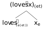
The leaves of the tree \(\tcon{loves}{(e(et))}\) and \(x_{e}\) are validated by Clause (1), while application of the former to the latter to form the root of the tree, , is validated by Clause (2). Now we take a further step and apply the function we obtained in to another item from our vocabulary, this time a constant rather than a variable:
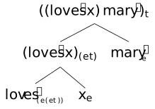
Our type system says that the expression at the root of is of type \(t\), which means it must stand for something that can be true or false. An approximation to this formal expression from natural language would be Mary loves it, him or her. The variable acts like a pronoun as mentioned above. And as in the case of natural language pronouns, we cannot decide on the truth value of the expression unless we know who or what the variable (or pronoun) stands for.
So far we made use of Clauses (1) and (2) of . Now let us see Clause (3) in action.
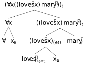
What we have here is an approximation to the sentence Mary loves everything.
In a similar fashion, we can invite our connectives into the business. Connectives will also be curried functions, so that they can be applied to their arguments one by one. For instance, the conditional will be applied to its antecedent and consequent one by one, resulting in the following equivalence to standard logical notation:
\[\begin{align*} ((\to \alpha)\beta) \equiv \alpha\to\beta \end{align*}\]Here is a representation corresponding to For any individual, if Mary loves him or her, then there is someone who gets broken:
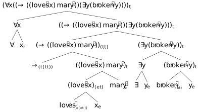
The formulas in their current forms are quite hard to read. One way to make them more readable is to agree on a convention to eliminate some parentheses. From now on we agree that in function application (i) outermost parentheses are omitted, and (ii) application associates to left. The first is easy to grasp: \(((fx)y)\) becomes \((fx)y\). The second needs some time get used to. Assume you are given an expression with some of its parenthesis are removed. Left association means that in restoring the parentheses back, you start from the two left most expressions, without looking into parentheses you encounter when counting the left-most two. Here are a couple of examples:
\[\begin{align*} x\cnct y \cnct z &\equiv& ((xy)z) & \\ x(yz) &\equiv& (x(yz)) &\\ x(yz)w &\equiv& ((x(yz))w) & \end{align*}\]Let us now apply these parentheses elimination conventions to ; observe that the type decorations goes away with the outer parentheses, you need to mentally keep track of them:
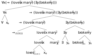
Semantics
Now it is time to give a semantics to our formal language \(L\). But before we embark on that task let’s preempt a nasty confusion of terminology. Below, we will use the term domain in a sense different from the usual one. The usual sense of the term is “the set of input values of a function”; but we will use it in a second sense, according to which the domain of a function \(f\) is the the set of all functions that has the same type as \(f\). In this extended sense, the domain of the function \(f(x)=x^2\) is the set of all functions from \(\mathbb{R}\) to \(\mathbb{R}\). The sense will also apply to non-functional objects.
First we define a model. A model \(\mathcal{M}\) is a tuple \(\langle D_e,D_t,I\rangle\), where \(D_e\) is the domain of individuals (i.e. a set of \(e\) type entities), \(D_t\) is the domain of truth values (usually ${0,1}$), and \(I\) is the interpretation function. We need some more notation to understand the mechanics of \(I\).
Given two sets \(X\) and \(Y\), \(X^Y\) denotes the set of all functions defined from \(Y\) to \(X\).
The notation is motivated by the fact that given two sets \(X\) and \(Y\) with cardinalities \(m\) and \(n\), respectively. There exists \(m^n\) functions from \(Y\) to \(X\).
Given a model \(\mathcal{M}=\langle D_e,D_t,I\rangle\), the domain of any type of objects can be denoted using . For instance, the domain of functions from entities to truth values is \(D_t^{D_e}\) or \(\{0,1\}^{D_e}\). For the domain of functions of type \((e(et))\) you will have \((\{0,1\}^{D_e})^{D_e}\), or for \(((et)t)\) you will have \(\{0,1\}^{(\{0,1\}^{D_e})}\), and in general the domain of functions of type \(\smtyp{\alpha}{\beta}\) is \(D_{\beta}^{D_{\alpha}}\).
For a model \(\mathcal{M} = \langle D_e, D_t, I \rangle\) to be a model for a language \(L\), the interpretation function $I$ should be able to return a value for all the constants (logical and non-logical) of \(L\) from the domain corresponding to the type of the constant. In other words, \(I\) needs to be an effective dictionary for the vocabulary of \(L\).
The interpretation function that comes with the model takes care of constants of our language; how about the variables? The variables – pronouns of \(L\) – are handled via the environment for evaluation, a function that maps variables of the language to corresponding objects in the model. Like the interpretation function \(I\), the environment, denoted by \(g\) maps each variable to an object with the same type. The fundamental difference between \(I\) and \(g\) is that the former is fixed by the model and does not change during the course of evaluation; the environment on the other hand is dynamic, it gets extended during evaluation. We define the extension of an environment as follows:
Given an environment \(g\), a variable \(x\), and a constant \(c\), an extension of \(g\) is the function denoted as \(\fnex{g}{x}{c}\) which is exactly like \(g\) possibly except that it maps \(x\) to \(c\).
It is time to state the semantics of \(L\) with respect to a model \(\mathcal{M}\) and an environment \(g\). You can think of evaluation as a higher order function denoted by double pipes: \(\interp{\psi}_{\mathcal{M},g}\) stands for the semantic evaluation of the expression \(\psi\) with respect to \(\mathcal{M}\) and \(g\).
- \(\interpp{\alpha} = g(\alpha)\), if \(\alpha \in V\)
- \(\interpp{\alpha} = I(\alpha)\), if \(\alpha \in C \cup K\)
- \( \interpp{(\alpha\beta)} = \interpp{\alpha}(\interpp{\beta}) \)
- \(\interpp{(\forall \alpha_{\pi} \beta)} = 1\) iff for all \(d \in D_{\pi}\), \(\interp{\beta}_{\mathcal{M},\fnex{g}{x}{d}} = 1\)
- \(\interpp{(\exists \alpha_{\pi} \beta)} = 1\) iff there is at least one \(d \in D_{\pi}\), \(\interp{\beta}_{\mathcal{M},\fnex{g}{x}{d}} = 1\)
Example
Let’s clarify over an example. Assume we were able to transform the sentence Whenever Mary loves someone, there is someone who will be jealous of the person Mary loves into the following logical form:
\[\begin{align*} \interpp{\forall x (\to (loves'\cnct x\cnct mary')\cnct (\exists y (jealous'\cnct x\cnct y)))} \end{align*}\]Any propositional expression like this can be either true or false with respect to a model. Therefore, we need to specify a model.
Here is our model \(\mathcal{M}\) and the environment \(g\):
\[\begin{align*} D_e = & \{\mtob{mary,pedro,rosinante}\} \\ D_t = & \{1,0\}\\ I = & \{(mary',\mtob{mary}), (pedro',\mtob{pedro}),\\ & (loves',\{(\mtob{mary},\{(\mtob{rosinante}, 1), (\mtob{pedro}, 1), (\mtob{mary}, 0)\}),\\ & \quad\quad\quad\quad (\mtob{pedro}, \{(\mtob{rosinante}, 0), (\mtob{pedro}, 1), (\mtob{mary}, 0)\}), \\ & \quad\quad\quad\quad (\mtob{rosinante}, \{(\mtob{rosinante}, 0), (\mtob{pedro}, 0), (\mtob{mary}, 1)\})\}), \\ & (jealous',\{(\mtob{mary},\{(\mtob{rosinante}, 0), (\mtob{pedro}, 1), (\mtob{mary}, 0)\}),\\ & \quad\quad\quad\quad (\mtob{pedro}, \{(\mtob{rosinante}, 1), (\mtob{pedro}, 0), (\mtob{mary}, 0)\}), \\ & \quad\quad\quad\quad (\mtob{rosinante}, \{(\mtob{rosinante}, 0), (\mtob{pedro}, 0), (\mtob{mary}, 1)\})\})\}\\ g = & \{(x,\mtob{rosinante}),(y,\mtob{rosinante})\} \end{align*}\]We do not provide the interpretations of logical constants, which are taken to be the standard logical connectives.
The first invoked clause of is (4):
\[\begin{align*} & \interpp{\forall x (\to (loves'\cnct x\cnct mary')\cnct (\exists y (jealous'\cnct x\cnct y)))} = 1 \text{ iff }, &\\ & \text{for all } d \in D_e,\quad \interp{(\to (loves'\cnct x\cnct mary')\cnct (\exists y (jealous'\cnct x\cnct y)))}_{\mathcal{M},\fnex{g}{x}{d}} = 1 \end{align*}\]We start iterating over \(D_e\), replacing \(x\) with a model-theoretic object in \(D_e\) and checking whether we obtain 1 as result. First,
\[\begin{align*} \interp{(\to (loves'\cnct x\cnct mary')\cnct (\exists y (jealous'\cnct x\cnct y)))}_{\mathcal{M},\fnex{g}{x}{\mtob{mary}}} \end{align*}\]This invokes clause (3):
\[\begin{align*} \interp{(\to (loves'\cnct x\cnct mary')}_{\mathcal{M},\fnex{g}{x}{\mtob{mary}}} (\interp{(\exists y (jealous'\cnct x\cnct y))}_{\mathcal{M},\fnex{g}{x}{\mtob{mary}}}) \end{align*}\]To handle this function argument form, let us first compute the function part \(\interp{(\to (loves'\cnct x\cnct mary')}_{\mathcal{M},\fnex{g}{x}{\mtob{mary}}}\), which is itself a function application, invoking clause (3) again:
\[\begin{align*} \interp{\to}_{\mathcal{M},\fnex{g}{x}{\mtob{mary}}} (\interp{(loves' x\cnct mary')}_{\mathcal{M},\fnex{g}{x}{\mtob{mary}}}) \end{align*}\]Now evaluate \(\interp{(loves' x\cnct mary')}_{\mathcal{M},\fnex{g}{x}{\mtob{mary}}}\), invoking clause (3):
\[\begin{align*} \label{lovesxmary} \interp{(loves' x)}_{\mathcal{M},\fnex{g}{x}{\mtob{mary}}} (\interp{mary'}_{\mathcal{M},\fnex{g}{x}{\mtob{mary}}}) \end{align*}\]Evaluate \(\interp{(loves' x)}_{\mathcal{M},\fnex{g}{x}{\mtob{mary}}}\), once again invoking clause (3):
\[\begin{align*} \label{lovesx} \interp{loves'}_{\mathcal{M},\fnex{g}{x}{\mtob{mary}}} (\interp{x}_{\mathcal{M},\fnex{g}{x}{\mtob{mary}}}) \end{align*}\]Evaluate \(\interp{x}_{\mathcal{M},\fnex{g}{x}{\mtob{mary}}}\), invoking clause (1):
\[\begin{align*} \interp{x}_{\mathcal{M},\fnex{g}{x}{\mtob{mary}}} = \fnex{g}{x}{\mtob{mary}}(x) = \mtob{mary} \end{align*}\]We also have the following by clause (2),
\[\begin{align*} \interp{loves'}_{\mathcal{M},\fnex{g}{x}{\mtob{mary}}} = I(loves') \end{align*}\]the evaluation step yields a function from \(e\) type objects to \(t\) type objects:
\[\begin{align*} I(loves') (\mtob{mary}) \\ = \{(\mtob{rosinante}, 1), (\mtob{pedro}, 1), (\mtob{mary}, 0)\} \end{align*}\]We have,
\[\begin{align*} \interp{mary'}_{\mathcal{M},\fnex{g}{x}{\mtob{mary}}} = I(mary') = \mtob{mary} \end{align*}\]Feeding this into its function, we get 0 as the value. Feeding 0 to the interpretation of \(\to\) would yield the function \(\{(0,1), (1,1)\}\). The next task is to compute the value for the consequent of the conditional with the extended environment and completing the iteration for \(x\mapsto \mtob{mary}\). The iteration has to go on until we are out of objects in \(D_e\). The completion of the evaluation is left as an exercise.
This was a brief and dense introduction to model-theoretic interpretation. It aimed to introduce how to define a semantics for a formal language that can be used as a logical form for natural language expressions. The research in natural language morphosyntax-semantics correspondence concentrates on how to map natural language expressions to logical forms. In such a setting logical forms serve an intermediary ground between form and meaning, just like intermediary languages and representations used in translating high-level programming languages to machine executable code. There are, broadly speaking, two camps that differ in the role they confer to intermediary representations. For one camp, the logical form is theoretically superfluous. According to this camp, semantic theory is a direct mapping from forms to model-theoretic objects, and logical form is there only to make this mapping more readable, or less complex to track, contributing nothing to the explanatory power of the theory. The other camp, on the other hand, takes logical form to be an essential part of the theory, where certain principles and mechanisms are defined at the level of logical form. In either case, the interpretation of logical forms has to be understood and internalized by semanticists, although it will not be part of their regular research practice. This paragraph will be justified.
-
If you are interested in the relation between the language we speak and the way we experience the world, check Sapir-Worf thesis and its critiques. ↩
-
By the way, we’ve been acting as if the elements of \(T\) stand on solid rock. But, do they? What are those expressions? Are they just colors, patches of them, lamps on the post, spectral ranges? ↩
-
This is so only in principle. No one, I guess, consciously thinks of the regulation every time they stop at a red light; but everyone, I guess, when asked, will cite the regulation as part of the reason why they stopped. ↩
-
It is hard to resist the feeling that you have access to the meaning of the languages you competently speak – we know a great deal about the meaning of words, don’t we?. But, the knowledge you have conscious access to is world (or conceptual) knowledge, rather than grammatical knowledge. As you advance in semantics, you will get much clearer on the difference. ↩
-
Given a set \(A\) and an operation \(f\), the closure of \(A\) under \(f\) is the smallest set that contains whatever you can get by zero or more applications of \(f\) to elements of \(A\) and values computed in any of the previous applications. Remember our axiomatization of propositional logic, where we closed the set of axioms under two inference rules (modus ponens and substitution) to generate the non-finite set of the well-formed formulas of the system. ↩
-
Linguistic convention italicizes expressions mentioned in running text. ↩
-
This is actually a provisional description, which I will adapt when I qualify the notion of sign below. ↩
-
You might be thinking that there is some object that stands as an answer to the question “What is a university?” Try for some time to describe that object. You will soon discover that this object is so slippery that you will be unable to come up with a description that tells what a university is in a satisfactory way. Don’t worry, you’ve just discovered the reason why good old-fashioned AI’s explicit knowledge representation efforts have miserably failed. ↩
-
Lewis (1979) “General Semantics”. ↩
-
Tractatus Logico-Philosophicus, 4.024. ↩
-
See Janssen (1997) for the problems with this naming. ↩
-
Think about the concept of sibling. If we put aside the notion of half siblings (Tr. üvey kardeş), we would think that it is a transitive and symmetric relation. But this causes a problem, can you see what? (Thanks to Omer Mert Coskun ) for pointing this out. ↩
-
We will reap the benefits on the computation side. ↩
-
Named after Haskell Brooks Curry, one of the inventors of the concept. Programming languages Haskell, Brook and Curry are also named after him. ↩